Case Study
Modular LiDAR SLAM Framework
A modular, sensor-agnostic 3D LiDAR SLAM framework for ROS2 that pairs Small-GICP scan-to-map odometry with Scan Context and Euclidean loop closure in the back end. Validated in Gazebo simulation and on a CSIR Voyager UGV across indoor and outdoor campus datasets, with sub-5 cm end-to-end error and real-time performance.
Problem
Real-time LiDAR SLAM is essential for autonomous mobile robots that need to perceive, plan and navigate in unknown environments. Research has made strong progress on LiDAR odometry and on loop closure detection separately, but far less work goes into combining them into one complete, deployable framework.
Existing systems also tend to share a few limitations. Many rely on computationally heavy algorithms that do not suit resource-constrained platforms. Loop closure is often an afterthought, typically a naive Euclidean distance check that fails once drift builds up. And popular feature-based methods such as LOAM, LeGO-LOAM and LIO-SAM are tuned for feature-rich urban scenes and tied to particular sensors, so they generalise poorly to places like mines or forests, or to different robot platforms.
Approach
The guiding principle was modularity: odometry and loop closure should be interchangeable components, not a tightly coupled pipeline. The system is a ROS2 package split into two independent nodes. A front end handles LiDAR odometry and sensor integration, and a back end handles loop detection and pose graph optimisation. The two talk over a custom message carrying the refined pose, the keyframe point cloud in the robot frame, and the distance travelled, so the fast front end never waits on the slower back end.
The framework is sensor agnostic and can run on LiDAR alone. When wheel odometry or an IMU is available, it fuses them for a better initial guess and for motion correction. The loop closure modules do not depend on the odometry method, so other registration or place-recognition algorithms can be swapped in without touching the rest of the architecture.
Technical Details
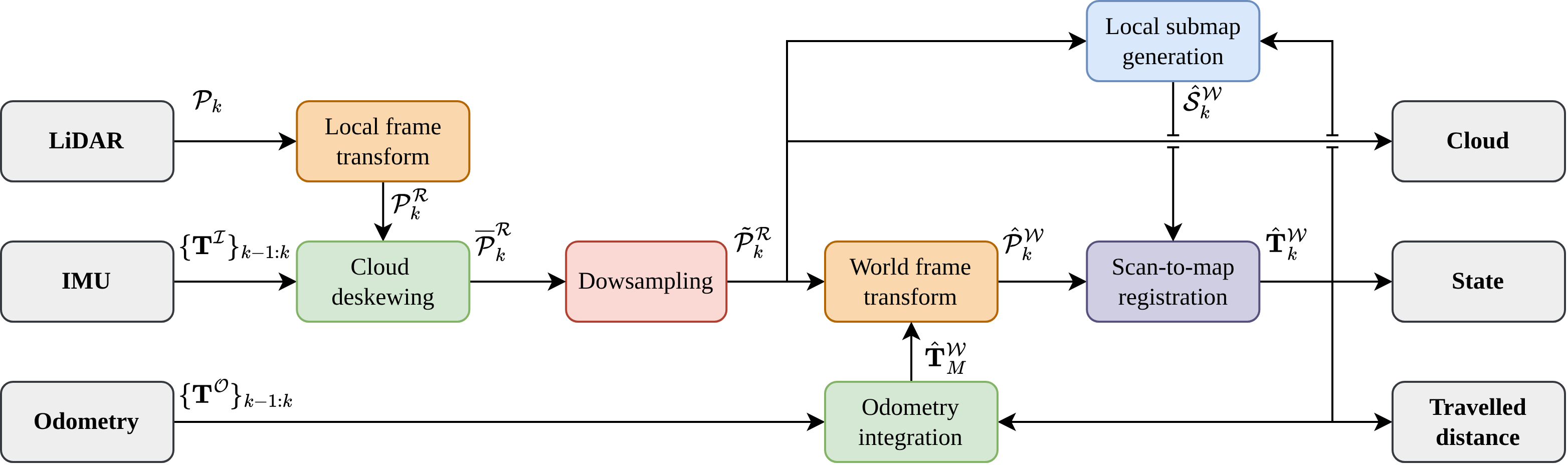
Front end: each scan is transformed into the robot frame using the LiDAR extrinsics, deskewed with IMU measurements from the scan period, and voxel-downsampled. An initial pose prior comes from wheel odometry or a constant-velocity model. The scan is then registered against a local submap using Small-GICP's voxelised GICP (VGICP). The submap is a voxel grid built from a configurable sliding window of past scans, with each voxel modelled as a Gaussian. Minimising the Mahalanobis residual between corresponding voxel pairs gives a correction transform that is applied to the prior to produce the globally refined pose.
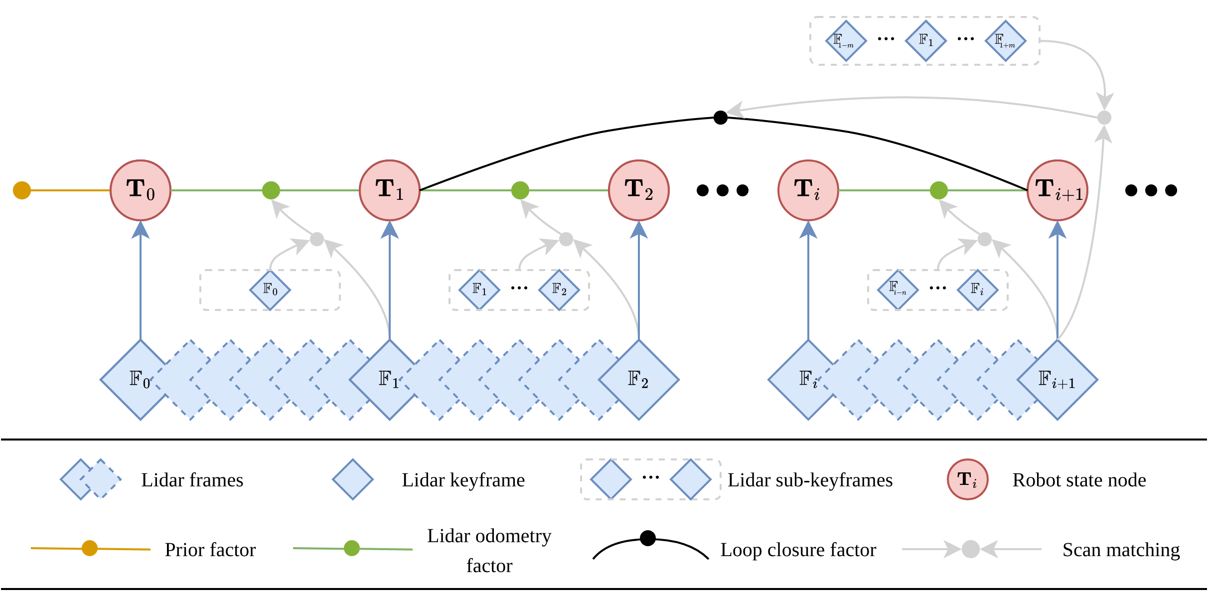
Back end: two loop closure detectors run side by side. A Euclidean distance check is cheap and can catch loops approached from any direction, but it becomes unreliable under drift. Scan Context builds an egocentric 2D polar descriptor from the maximum point height in each sector and matches it against a database, so it is independent of odometry and robust to drift, though only invariant to yaw. Candidates from both detectors are confirmed by scan registration and a fitness threshold. Confirmed loops are added to a g2o factor graph alongside a prior factor and LiDAR odometry factors between keyframes. Each new loop triggers Levenberg–Marquardt optimisation, after which the stored local clouds are re-projected to update the global map.
Outcome
In Gazebo simulation, evaluated against ground truth with evo, the system reached an absolute trajectory RMSE of 0.022 m on the Testpen environment (45 m trajectory) and 0.050 m on the Cave environment (205 m trajectory, 2 m elevation change). Average computation time was 5.8 ms and 11.0 ms per frame respectively.
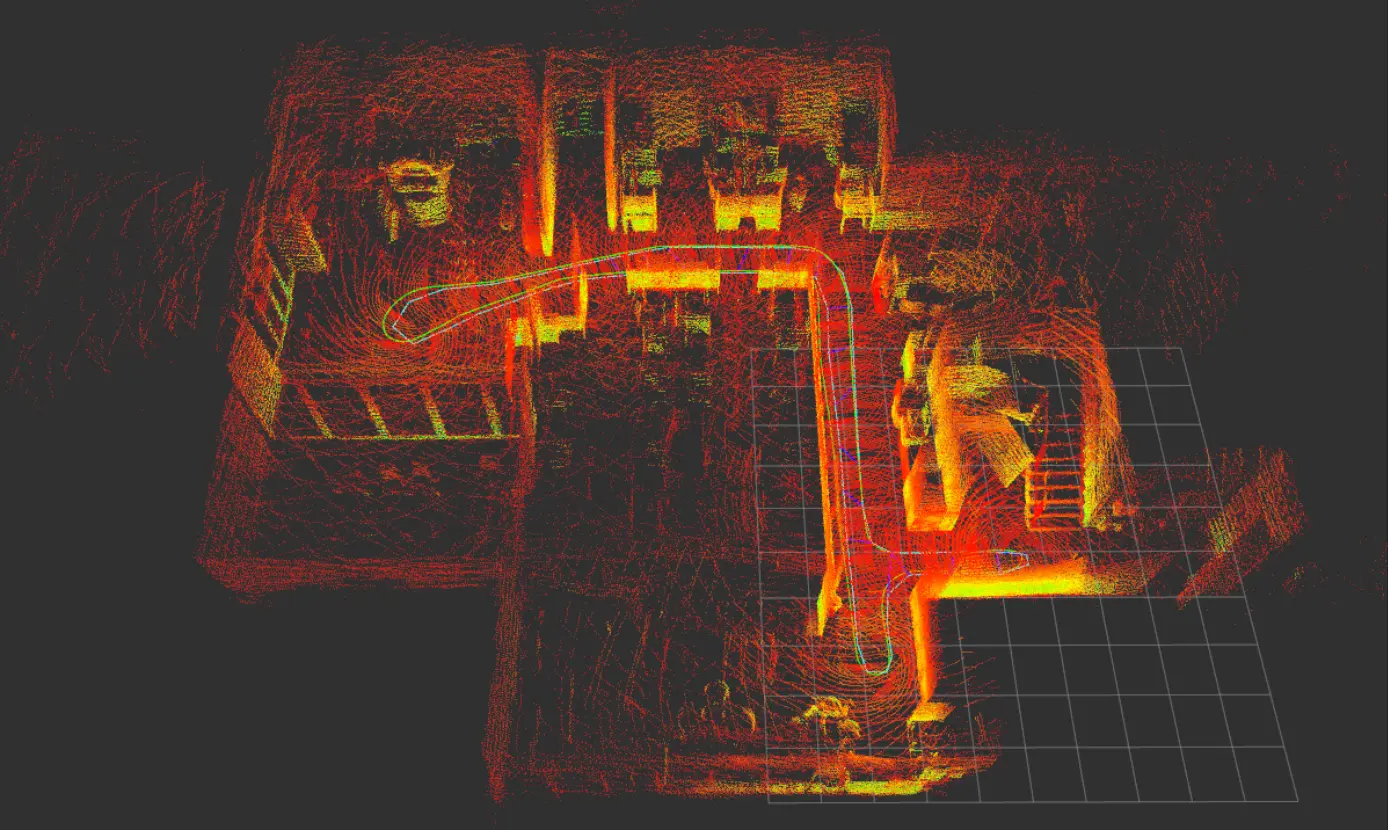
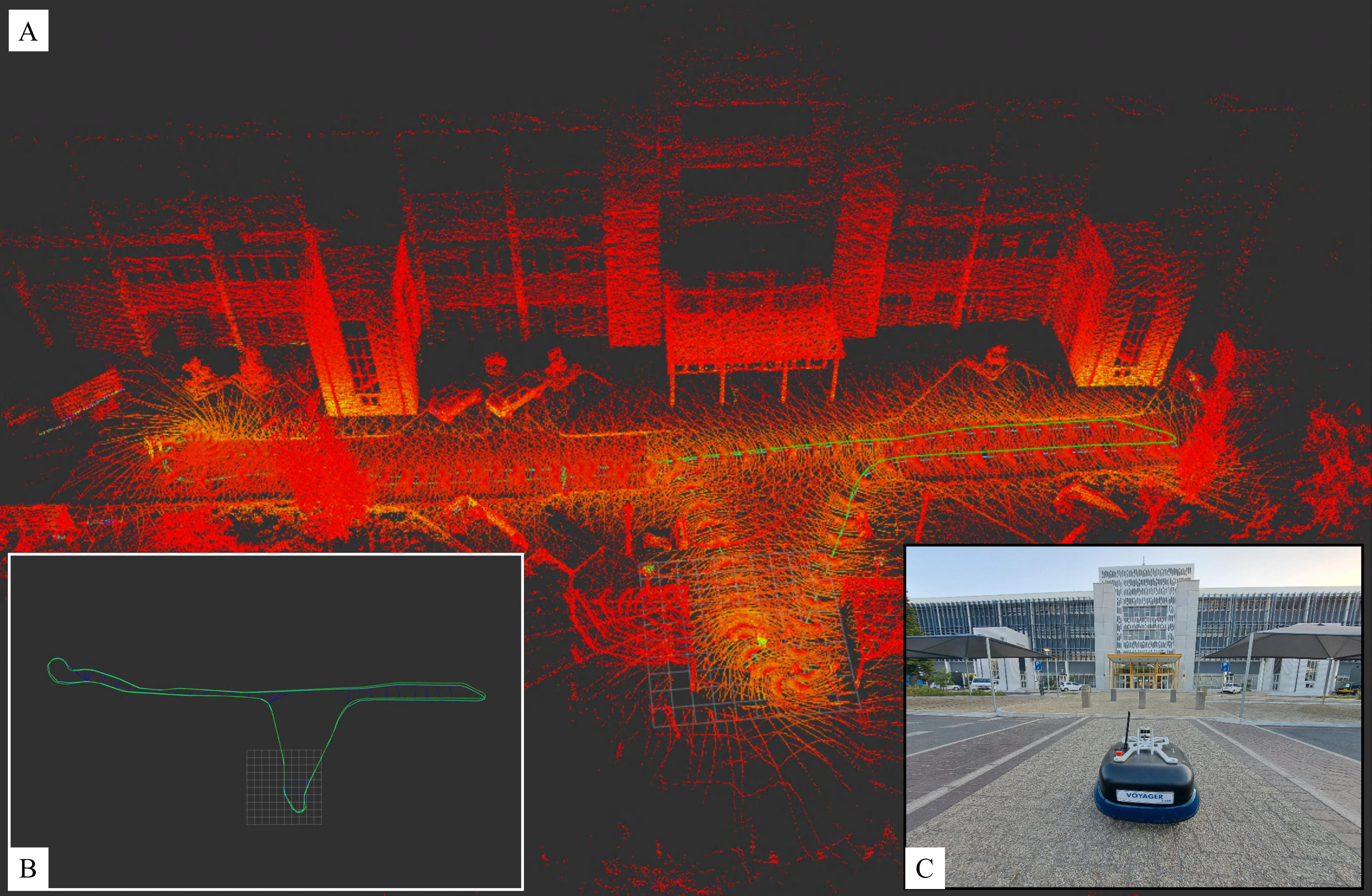
On real data collected with the CSIR Voyager UGV (Ouster OS0-32, Xsens MTi-630 IMU, wheel encoders), the framework mapped four campus datasets of up to 190 m using the same front-end parameters throughout. End-to-end translational error was 0.022 m (Laboratory), 0.031 m (Hallway), 0.050 m (Parking) and 0.133 m (Walkway). The system detected up to 50 loop closures per run and averaged 10 to 44 ms per frame, comfortably real-time for a 10 Hz LiDAR. The two loop detectors caught different loops, confirming that combining them works better than either alone.
The work was written up as a paper with C. Fisher at Stellenbosch University. Planned next steps are GPS and camera integration and evaluation on ground-truth benchmarks such as Newer College.
Media
Tech Stack